Graph View on Automatic Differentiation

Few people are familiar with the graph view on automatic differentiation, although it is quite helpful for understanding what automatic differentiation (AD) actually does. The underlying idea is to frame AD as an operation on the computational graph. This short blog article tries to give an overview over this concept called vertex elimination and tries to describe in detail how it works. Consider a simple function $f$ that maps two inputs to two outputs:

$$ f(x_1, x_2) = \begin{pmatrix} \log \sin x_1x_2 \\ x_1x_2 + \sin x_1x_2 \end{pmatrix} $$

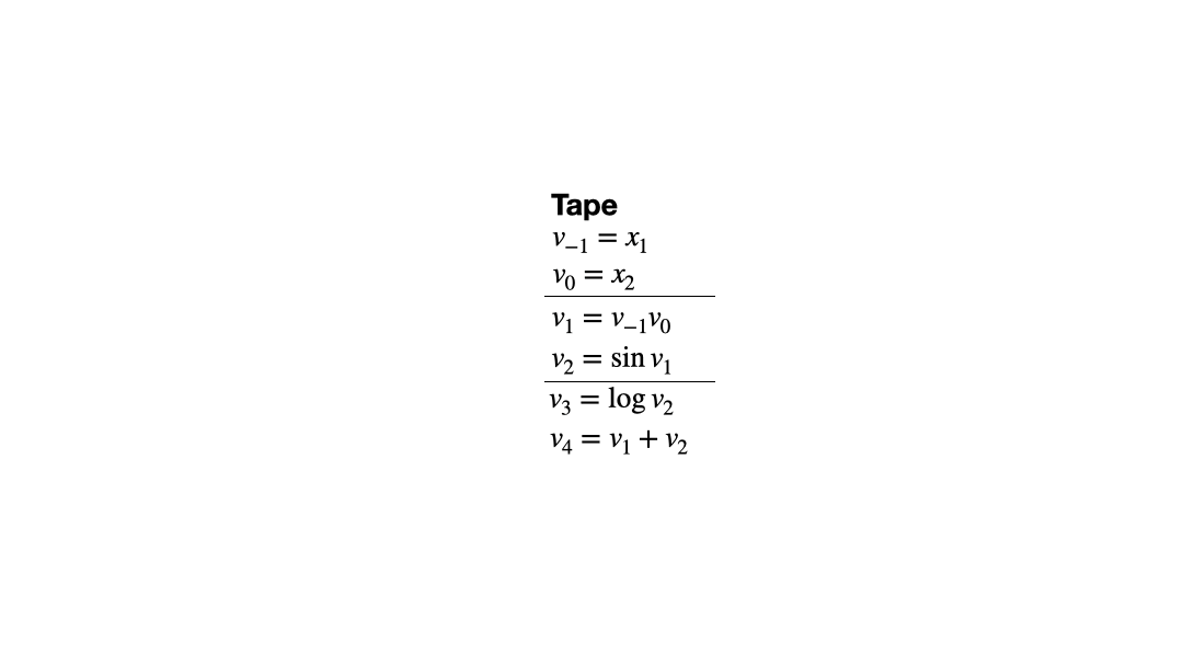
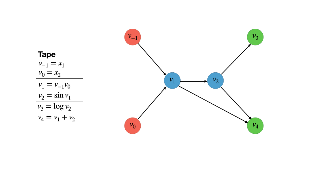
The first thing we need is the computational graph. We obtain this graph by first dissecting the function $f$ into a sequence of elemental operations like additions, multiplications, logarithms etc. This step is always part of every AD algorithm/method because for these simple functions we know the exact (partial) derivatives. With the chain rule, we can then assemble the Jacobian of $f$ from these simple elemental partial derivatives. Most AD algorithms then differ in the order in which the chain rule is applied, e.g. forward-mode AD vs. reverse-mode AD (aka backpropagation). After we have dissecting $f$ into its elemental operations we store them in sequential order in a list called the Wengert List or the Tape (see figure 1). Every elemental operation outputs an intermediate variable $v_i$ which is then fed to the next operation.

Figure 1: The tape is obtained by simply tracing through the equation and identifying the elemental operations where we know the derivatives analytically. Then we write the equation as a sequence of said elemental operations.

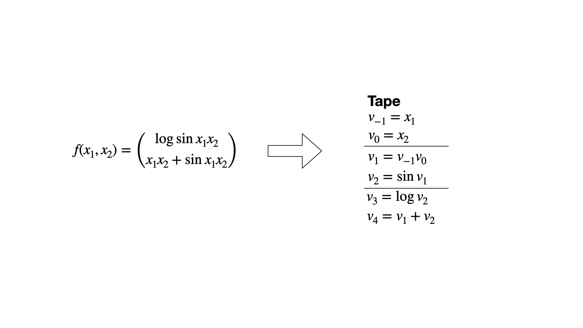
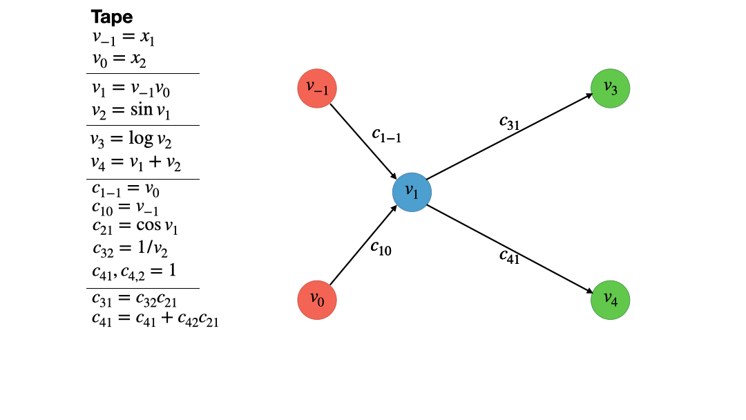
Not that the naming convention is a bit weird as we index the using negative numbers up to 0, while the first elemental operation is indexed using 1. The reason for this will become clear in just a moment. To construct the computational graph, we now draw a bunch of vertices, one for each input variable, operation and output variable. The edges that connect the vertices just represent the data dependencies of the inputs, operations and outputs. For example, since the addition depends on both input variables, $x_1=v_{-1}$ and $x_2 = v_0$, the vertex $v_1 = v_{-1}v_0$ has two edges connecting them. Since the vertex $v_1$ is involved in computing $v_2$ and $v_4$ it has to edges emanating to these vertices, making a total of two ingoing and two outgoing vertices. Note that input vertices are red and only represent numbers, while intermediate and output vertices are blue and green respectively. The latter two only differ in the fact that an output vertex has no outgoing edges. Figure 2 provides a visual account of the computational graph creation.

Figure 2: This animation shows how the computational graph is created from the tape that stores the elemental operations that make up function f. Input variables are red, intermediate elemental operations and corresponding variables are blue and output vertices are green.

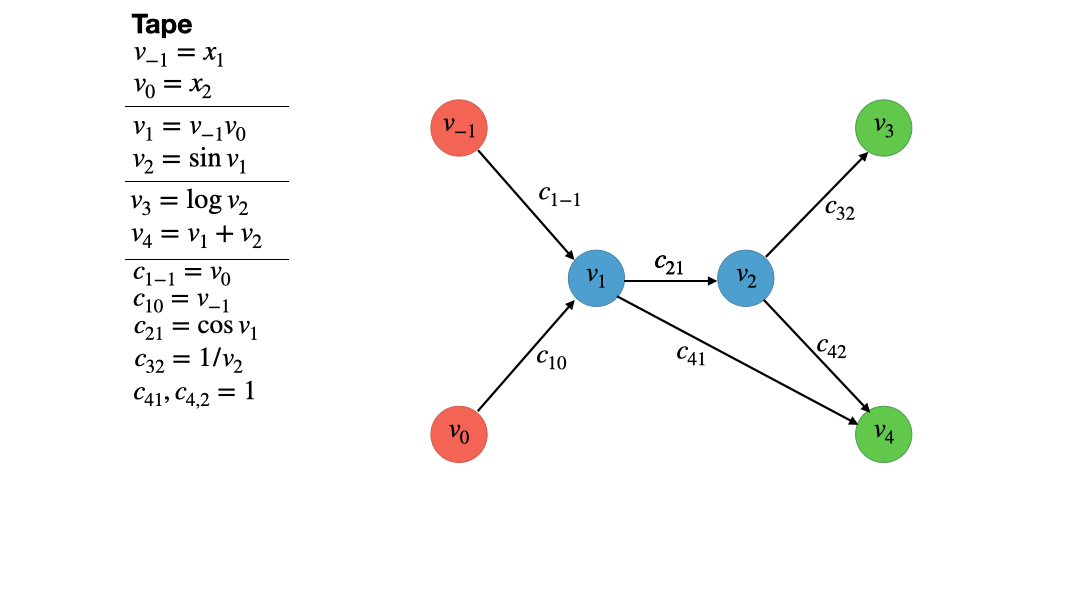
The first step towards the vertex elimination algorithm is to populate the edges of the graph with partial derivatives of the destination vertex with respect to the source vertex. For example for the edge going from vertex $v_{-1}$ to vertex $v_1$, we would compute
\(c_{ji} = \dfrac{\partial v_1}{\partial v_{-1}} = \dfrac{\partial}{\partial v_{-1}} (v_{-1}v_0) = v_0\)
and add this to the edge as an associated value. We introduce the shorthand $c_{ji}$ for the partial derivative value associated with the edge going from $i$ to $j$. Note that we add the computed partial derivatives to the tape as well. In general, we will utilize the tape as a record keeping devices that stores all the operations that have been computed “on the graph”.

Figure 3: The animation demonstrates the population of the graph’s edges with partial derivatives. Note that for every computed derivative we add an entry to the tape.

Now it is time to describe the actual vertex elimination algorithm. For this, we take a look at the second intermediate (blue) vertex. It has one ingoing and two outgoing vertices. The vertex elimination rule for vertex $j$ now states:

For every ingoing edge of vertex $j$ we multiply the corresponding partial derivate $c_{ji}$ with every partial derivative of every outoing edge $c_{kj}$. For each of these products, we draw a new edge from the source vertex $i$ of the ingoing edge to the destination vertex $k$ of the outgoing edge and identify the associated partial $c_{ki} = c_{kj}c_{ji}$. If said edge already exist, we just add the values, i.e. $c_{ki} = c_{ki} + c_{kj}c_{ji}$. Finally we delete all edges connected to vertex $j$.

Figure 4 gives an animated example of how this works for our function $f$. Note that this is nothing else than locally applying the chain rule to vertices $i$, $j$ and $k$. As a quick illustration, look at the very simple graph $x \to g(x) \to f(g(x))$. The ingoing edge has the derivative $g’(x)$ associated with it while the outgoing edge has the associated value of $f’(g(x))$. The application of the vertex elimination rule would give $x \to f(g(x))$ where the new edge directly connecting $x$ and $f(g(x))$ has the value $f’(g(x))g’(x)$.

Figure 4: Vertex elimination of vertex 2. Red dotted edges are the ones that are newly created or overwritten. Note how vertex 2 is completely disconnected from the graph after the application of the vertex elimination rule and thus deleted.

After eliminating vertex 2, we eliminate vertex 1 with the same procedure. Figure 5 shows how this is done. After vertex one is eliminated, there are no intermediate, blue vertices left. In fact we have what is called a bipartite graph. What is this good for? There exists a series of proofs [1] that show that if we apply the vertex elimination rule to a computational graph and make it bipartite, the values $c_{ji}$ on its edges are exactly the elements of the Jacobian of our function. This shows that vertex elimination of all intermediate (blue) vertices yields and algorithm that allows us to compute the Jacobian of a function $f$. As in every good textbook we leave the verification of this statement for the given example to the reader. No really, just do it!

Figure 5: Elimination of vertex 1 using the vertex elimination rule. Note how we end up with a bipartite graph after vertex 1 is eliminated.

Note that the actual algorithm is not contained in the graph, but rather in all the operations and assignment that have been recorded on the tape. It is fairly easy to implement this sequence of operations in a language of your choice. But what is this good for? And why did we do the elimination order 2 then 1 (2, 1) instead of 1 then 2 (1, 2)? We start by answering the second question. Doing this is totally valid and one could easily do this. Another exercise for the reader maybe! In any case, the resulting algorithm will yield the same Jacobian but there is a big difference. If you look closely at the tape in figure 5, you see that the vertex elimination of order (2, 1) has incurred 6 multiplications and 1 addition (excluding the computation of the $f$ itself and the partial derivatives, only the accumulation). Doing the order (1, 2) will instead incur 8 multiplication and 2 additions! Aha, there is a difference in computational requirements depending on the elimination order. As a matter of fact, every vertex elimination operation incurs a certain number of multiplications and additions depending on which vertices have been eliminated before. Thus every order of elimination creates its own algorithm which we can extract from the tape and has its own computational cost. Vertex elimination is a systematic way to create tailored AD algorithms for a given function $f$, each with their own computational cost. Obviously, we would like to select the algorithm with the lowest computational cost. This is a NP-complete problem. I offer one solution which I called AlphaGrad. It can be found under this link.

Extensions

The way vertex elimination was described so far is actually very limited if you want to use it for production usecases. There are two possible extensions that make vertex elimination applicable to a wider range of problems.

1. Support for Vectors and Tensors In many modern applications, the function $f$ will have vector- or tensor-valued inputs, e.g. a neural network. While it would be mathematically possible to treat every value as a single input value, this would be cumbersome to do. A more viable approach instead would be to allow vertices to have vector- and tensor-valued derivatives, i.e. partial Jacobians. Then the multiplication of two partial derivatives becomes a contraction of two tensors instead. The addition remains the same. The important part of this is that many Jacobians have an internal sparsity structure that should be exploited when performing the contractions, because otherwise the gains through vertex elimination are quickly lost. More on that can be found in the AlphaGrad paper. If you want to play around with vertex elimination and even use vector and matrix-valued functions, have a look at my graphax package.

2. Other Metrics While counting the number of multiplications and additions is a nice theoretical way of judging an algorithms performance, they often only give a limited account of the actual performance. Instead, it might make more sense to select vertex algorithms with respect to actual runtime, memory use etc.

3. Edge and Face Elimination Vertex elimination is only one way to systematically construct AD algorithms. Edge elimination uses the same principle but for individual edges instead of whole vertices. Face elimination lifts the whole business to a whole level by introducing faces as objects that consist of multiple vertices and edges. Learn more about this in [1].

Sources

[1] Evaluating Derivatives. Griewank und Walther. 2008. SIAM.
[2] Optimizing Automatic Differentiation with Reinforcement Learning. Lohoff and Neftci. 2024. Proceedings of NeurIPS 2024.